Differentiation and Quadrature#
A vast number of applications such as the calculation of tangent vectors or areas lead to the problem of computing
for certain function \(f(x)\in C^k([a, b])\). Accurate evaluations would sometimes be difficult if an analytic expression is absent. Especially when the function values of \(f\) are only accessible at a finite number of nodes. Therefore, it is important to find simple yet effective methods to approximate the derivatives and integrals.
Extrapolation#
From the previous discussion, we already know that interpolation provides an estimate within the original observation range. The extrapolation is similar but aims to produce estimates outside the observation range. However, sometimes extrapolation may be subject to a greater uncertainty (see following example), one should use it only when an overestimate is hardly occurring.
Matplotlib is building the font cache; this may take a moment.
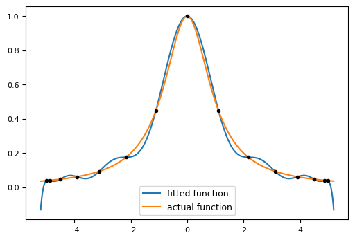
Fig. 7 Extrapolation behavior of polynomial fitting on Chebyshev nodes.#
Richardson Extrapolation#
Suppose there is a sequence of estimates \(A(h)\) depending on the parameter \(h\) smoothly, the limit \(A^{\ast} = \lim_{h\to 0^{+}} A(h)\) is the quantity to be computed. In practice, we only have access to \(A(h)\) for a few values of \(h\). Using these values to estimate \(A^{\ast}\) is a typical problem in extrapolation.
The basic idea behind Richardson extrapolation is to use polynomial interpolation with a sequence of nodes \(h_j\to 0\). Suppose that the function \(A(h)\) admits the following asymptotic expansion:
for any \(h > 0\) and \(k\ge 0\). Then \(A^{\ast} = a_0\) and \(A(h) = A^{\ast} + \cO(h^{\gamma})\). Suppose we have access to the values \(A(h_0),\dots, A(h_n)\), then this uniquely determines a polynomial \(f_n\in\Pi_n\) and \(f_n(h_j^{\gamma}) = A(h_j)\). We will approximate \(A(0)\approx f_n(0)\). The computation of \(f_n\) follows the construction of the Newton form.
Lemma 6 (Richardson Extrapolation)
Suppose \(h_j\) can be represented as
for some adjustable parameter \(\hbar\) and scaling constants \( 1 < t_0 < t_1<\dots < t_{n-1}\). Then
Proof. We view \(A(h)\) as a polynomial with respect to \(h^{\gamma}\) of degree \((n+1)\) with an addition perturbation \(\cO(h^{(n+2)\gamma})\). Then we have the following.
Let \(\tilde{f}_n\) be the interpolation polynomial of degree \(n\) to \(p_{n+1}\),
where \(p[x, h_0, h_1, \dots, h_n]\) is the coeffimathcal{I}ent of the leading power in \(p_{n+1}\), \(a_{n+1}\). Thus,
Here we use the result for the stability of polynomial interpolation in earlier chapters. Therefore,
Here the Lebesgue function at zero \(\lambda_n(0)\) is
which is independent of \(\hbar\).
The Richardson extrapolation considers the special choice of \(t_j = t^j\) for some \(t > 1\). The error estimate then is
There are easier ways to calculate the Richardson extrapolation using the following expansion.
Let \(A_1(h) = \frac{A(h) - t^{\gamma} A(\frac{h}{t}) }{1 - t^{\gamma}} \), we obtain the first iteration result as
then follow the same idea, we cancel the \(\cO(h^{2\gamma})\) term by
Therefore by taking \(A_2(h) = \frac{A_1(h)- t^{2\gamma} A_1(\frac{h}{t^{2\gamma}})}{1 - t^{2\gamma}}\), the second iteration satisfies
However, such a process may not constantly refine the approximation due to the potentially fast-growing constant in the \(\cO\) notation.
Aitken Extrapolation#
Alexander Aitken rediscovered Aitken extrapolation, which has been used to accelerate a sequence’s convergence.
Given a sequence \(S = \{s_n\}_{n\ge 0}\), the Aitken extrapolation generates a new sequence
A more stable formulation (why?) is written as
where \(\Delta\) is the forward difference operator that \(\Delta s_n = s_{n+1} - s_n\). It is not difficult to see that Aitken extrapolation can accelerate linearly convergent sequences.
Theorem 18
Assume that the sequence \(S = \{s_n\}_{n\ge 0}\) satisfies
Then the accelerated sequence \(AS\) converges faster than \(S\).
Proof. Let \(\rho_n := \frac{s_{n+1} - \mu}{s_n - \mu}\), without loss of generality, we assume \(\lim_{n\to\infty} \rho_n = \rho\).
By the definition of the acceleration formula, we obtain
For sufficiently large \(n\), we have \(\rho_n \approx \rho\) and
Therefore
Remark 14
Let \( \eps_n := s_n - \mu\). If the error satisfies the following relation (common in most fixed-point iterations) $\(\eps_{n+1} = \eps_n (\rho + c_1 \eps_n + o(\eps_n)),\)$ then
That is, \(| (AS)_{n} - \mu| = \cO( |s_{n} - \mu |^2 )\).
The Aitken extrapolation can be used to accelerate fixed-point iteration solving the root \(x^{\ast}\) for \(f(x)\). Steffensen’s method is a root-finding algorithm based on such an acceleration technique, the iteration is given by
If \(f\) is twice differentiable, then clearly the function \(g(x)\approx f'(x)\), which recovers the Newton-Raphson method asymptotically if \(f(x)\approx 0\).
Theorem 19
Suppose \(f'(x^{\ast})\in (-1, 0)\), then the order of convergence is 2 for Steffensen’s method.
Proof. Let us first point out the connection between Aitken extrapolation and Steffensen’s method. Denote \(x_0\) as the starting point, the intermediate values \(z_1 = x_0 +f (x_0)\) and \(z_2 =z_1 +f(z_1)\). The Aitken extrapolation finds
The convergence is linear when the iterates \(x_0, z_1, z_2\) are close to the root \(x^{\ast}\). Therefore, using the same derivation, we find
Remark 15
It should be noticed that Steffensen’s method evaluates \(f\) twice during each iteration, the same as Newton’s method (one for \(f\) and one for \(f'\), although the evaluation of \(f'\) is more expensive in practice). Each evaluation brings an order of \(1\) of convergence on average. From the viewpoint of efficiency, the secant method is preferred, since it only evaluates \(f\) once each iteration with an order of \(\frac{1+\sqrt{5}}{2}\) of convergence.
Wynn’s Epsilon Method#
Wynn’s \(\eps\) method [Wynn, 1956, Wynn, 1966] is another kind of extrapolation algorithm that is recommended as the best all-purpose acceleration method. It has a strong connection with Padé approximation and continued fractions. We will not cover the detailed derivation of the theory in this section. However, Wynn’s \(\eps\) method still has its limitations if the sequence converges to the desired value too slowly.
The algorithm is stated as follows.
Algorithm 4 (Wynn’s \(\eps\) Method)
Input: \(s_0, s_1, \dots, s_n,\dots\), which is a sequence converging to the desired quantity.
Output: \(\eps_{2l}^{(j)}\), \(j, l=0,1, \dots\).
For \(j = 0, 1, 2,\dots\), set
For \(j,k = 0,1,2,\dots\),
Example 5
It is known that \(\frac{\pi}{4}\) can be calculated by the asymptotic expansion:
at \(z = 1\). Define the function \(A(h)\) such that
Then the approximation error is \(\cO(h)\), which is very slow. Taking \(h=10^{-3}\) has around \(2\times 10^{-4}\) error. We test with two extrapolation algorithms.
Richardson Extrapolation. We take \(1/h = 250, 500, 1000, 2000\) and calculate that the Richardson extrapolation three times would result in almost machine premathcal{I}sion.
Wynn’s \(\eps\) method. We take the sequence
\[ s_k = \sum_{j=0}^k \frac{(-1)^j}{2 j + 1} \]as the truncated series at \(z = 1\). With about 20 terms, we already reached machine precision.
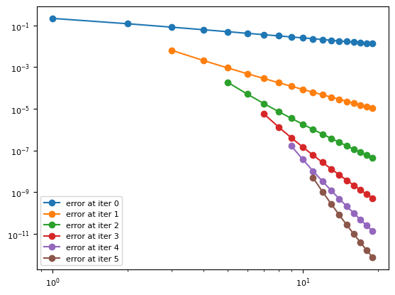
Fig. 8 Absolute error of \(\eps_{2l}^{(j)}\) for Wynn’s \(\eps\) method, \(0\le l\le 5\).#
Quadrature#
The numerical quadrature finds the value of an integral
from the function values at a finite number of points. We are mostly interested in the following quadrature formula
where \(x_j\) are the nodesand \(w_j\) are the weights. Similar to the numerical derivatives, we also define some terminologies. The formula \(\mathcal{I}_n\) is said to have degree \(k\) accuracy if \(\mathcal{I}_n\) is exact for all polynomials \(f\in\Pi_k\). Since the integration formula is linear, the exactness can be rephrased as
Interpolation Based Quadrature#
The interpolation-based idea is intuitive. Let \(q_n(x)\) be the interpolation polynomial on the nodes \(x_j\) with values \(f(x_j)\), \(j=0,1,\dots, n\), respectively. We define the quadrature by interpolation formula as
The above quadrature formula is exact for all degree \(n\) polynomials \(f\), therefore it has at least degree \(n\) accuracy.
Remark 16
We have seen that the \(L^{\infty}\) error between \(f\) and \(q_n\) could be large (e.g. Runge phenomenon) as \(n\to \infty\). So the nodes would be important as well for quadratures.
Using the Lagrange polynomials, we can represent
Then it is not difficult to derive
therefore the weights \(w_j = \int_0^1 \prod_{k=0, k\neq j }^n \frac{t - t_k}{t_j - t_k} dt\).
Example 6
The rectangle rule is the simplest, where we choose \(x_0 = \frac{a+b}{2}\) as the middle point. Then the quadrature rule writes
Such a rule is exact for any linear function, so it has a degree of accuracy of one. We can see that the degree of exactness could exceed \(n\). In the next chapter, we will see that the maximum degree of exactness for such a form is \(2n+1\).
Example 7
The trapezoid rule takes \(x_0 = a\) and \(x_1= b\).
One can check that this rule is exact for \(f(x) = 1, x\). Its degree of accuracy is one. It has a slightly larger constant in error estimate than the rectangle rule.
Example 8
The Simpson’s rule takes \(x_0 = a\), \(x_1 = \frac{a+b}{2}\), and \(x_2 = b\).
This rule is exact for \(f(x) = 1, x, x^2, x^3\), thus the degree of accuracy is three.